Sep 4, 2026

ML for Drone Delivery

Learn how to build a drone that can spot a safe place to land, using AI trained on aerial video to tell driveways apart from cars, roofs, and people.

Teaching a Drone Where to Land

A delivery drone hovering over a house has one question to answer before it lowers anything on a winch: where is it safe to put this? Ideally the answer is a driveway with nobody standing on it, no bike left across it, and no car parked in the middle. The answers you never want are the roof of the house or the hood of a car.

This tutorial walks you through the complete pipeline for an AI-powered drone delivery prototype, from raw aerial footage to a model running onboard and picking out a landing zone. You will capture video from a PX4 drone, extract frames into a dataset, annotate eight classes with polygon segmentation masks in Roboflow, train a YOLOv11 segmentation model in Google Colab, export it to TensorFlow Lite, and wire it into a MAVSDK Android app that draws detections over a live video feed. By the end you will have the full workflow required to move a computer vision model from drone imagery to an onboard system that can locate and center over a potential delivery zone. As usual, you can follow along with the written tutorial below or the video from the livestream.

Why Segmentation Instead of Object Detection

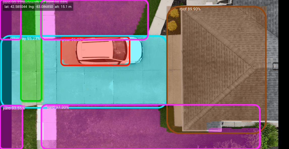
Object detection draws rectangles. That is fine when you only need to know that a car exists somewhere in the frame, and it has been the approach in several previous drone projects here. It falls apart when the question is whether a specific patch of concrete is clear enough to land on, because a bounding box around a driveway includes whatever grass, sidewalk, and shrubbery happen to sit in the corners of the rectangle.

Instance segmentation predicts precise object boundaries using polygon masks instead. The mask follows the actual edge of the driveway, so when the model reports a driveway and separately reports a car sitting on it, the geometry is accurate enough to reason about the space that remains. For picking a landing zone out of a suburban lot, that difference is the whole ballgame, and segmentation does a noticeably better job here than the object detection models used previously.

The Hardware

The cheapest setup we found that works is the Holybro PX4 development kit at around $530.

The kit does not include a camera, so budget for that separately. We found two options:

Siyi A8, $250. A gimbal camera, which is what these flights used.
Siyi HM30, $250

We also looked into the DEXI 5 from Droneblocks It’s one of the cheapest NDAA-compatible option at $2000+, and it comes with a basic camera. Buy it as a kit rather than assembled if you want to learn the hardware, which is worth the extra effort.

The drone frame we used was 3D printed from the old 3DR IRIS frame, a public domain STL file, which keeps the cost down and makes replacements easy when something breaks.

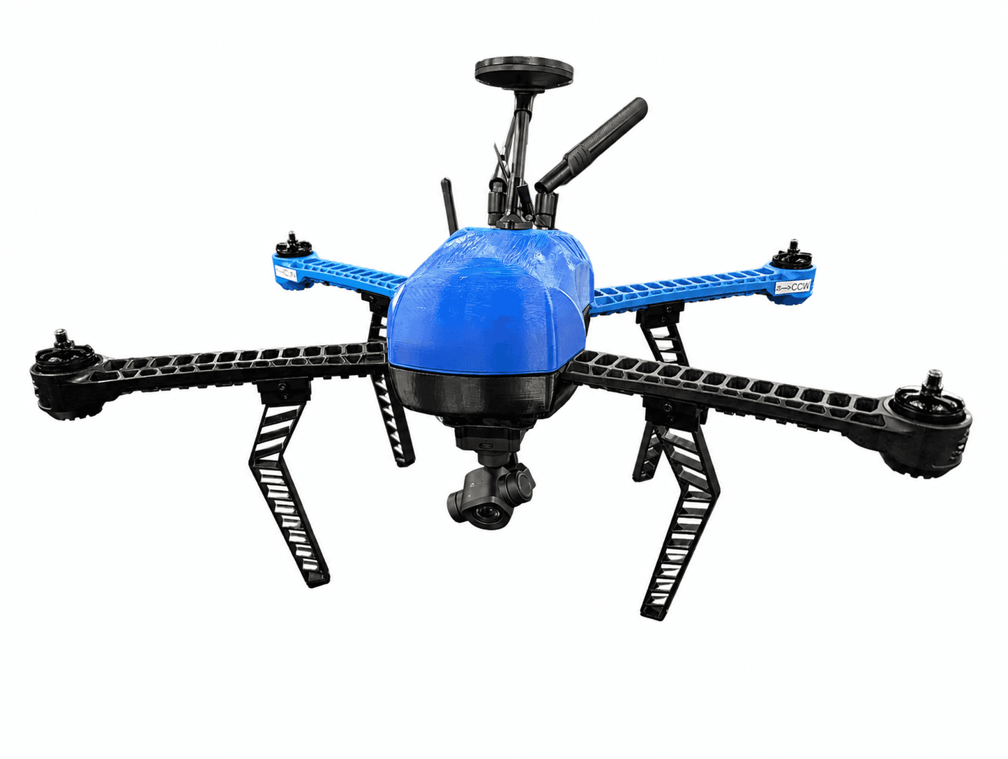
That build pairs the printed frame with a microhard radio, an orange cube flight controller, a Raspberry Pi for video streaming, and the Siyi A8 camera. The Raspberry Pi is there because the video telemetry has to reach the phone running the app, which is a separate path from the flight telemetry the radio carries.

The Pipeline

Eight steps take you from a drone in the air to a model picking landing zones:

Capture drone footage
Download the footage and extract image frames
Upload the images to Roboflow and annotate each class with polygon masks
Export the labeled dataset from Roboflow in YOLOv11 format
Train the model in Google Colab using the dataset
Evaluate model performance with mAP scores
Export the trained model to TFLite format
Deploy the TFLite model to a Google Pixel running the MAVSDK client

Note you can also store the images locally, but Roboflow makes sure you don’t lose track of them or they get locked into a single workstation.

The rest of this tutorial works through them one at a time.

Project Setup

Everything lives in the godfreynolan/drone_delivery repository:

extract_frames.py turns raw flight video into a folder of JPEG stills.
YOLO_Drone_Delivery_Training_(segmentation).ipynb is the Colab notebook that trains and exports the model.
android-client/ is a fork of the MAVSDK Java sample app with the detection pipeline added.

The frame extractor needs only OpenCV, which is the entire requirements.txt:

The training notebook installs its own dependencies inside Colab, and the Android client builds through Gradle in Android Studio. If something in the repo does not work for you, open an issue and it will get dealt with.

Capturing the Footage

Machine learning models get better as the problem gets narrower, so the guiding principle for data collection is to make the conditions as restrictive as you can. Fly the same drone, at the same height, with the same camera pointed the same direction every single time. Every variable you eliminate is one the model does not have to learn its way around.

In practice that means a short list of rules:

Select multiple residential neighborhoods so the dataset covers a diverse range of driveways, streets, and surrounding environments.
Fly at approximately 15 meters, about 49 feet, above ground level, and always fly at the same height. At 15 meters you are above most trees, power lines, and cable runs, and the scale of everything in frame stays consistent.
Set the camera gimbal to -90 degrees, straight down, for a nadir bird’s-eye view.
Record continuous high-resolution video over the selected neighborhoods.
Capture variety within those constraints: driveways, streets, parked vehicles, houses and rooftops, sidewalks, and surrounding terrain.

Try flying at different times of day and in different weather. Lighting is the variable that quietly ruins aerial datasets. A previous project used object detection to count cattle and sheep, with footage arriving from across the US, Ireland, New Zealand, and South Africa, and the lighting differences between California, Arizona, the Midwest, and New York were dramatic before you even left the country. Train for where you will actually fly. If you need footage from other cities, Fiverr and Upwork are good places to hire someone to fly for you, as long as they use the same camera.

The same advice applies to annotation, which is genuinely tedious work and a reasonable thing to outsource, provided somebody checks the results.

One more thing to plan for: this is a pipeline, not a one-time job. Every delivery flight you run afterwards is more training data, and feeding it back in is how the model keeps improving. Anyone who tells you their model is 100% accurate is lying.

Extracting Frames from Video

The model does not consume video. It consumes still images, so each frame goes to the network on its own with the question of which trained objects appear in it and where.

After the flights, transfer the .MP4 files off the drone and organize them into batch folders per session. A custom Python script then processes each video and saves individual frames as .jpg images. The interval matters: consecutive frames from the same flight are nearly identical, so annotating them is wasted effort. The seconds_between_frames variable controls the spacing, and at 5 seconds an 11-minute video yields roughly 135 images.

The script uses OpenCV to read the video files and write frames to an output folder:

import cv2
from pathlib import Path

video_folder = Path("videos4")
output_folder = Path("images4")
output_folder.mkdir(exist_ok=True)

seconds_between_frames = 5

image_count = 1

import cv2
from pathlib import Path

video_folder = Path("videos4")
output_folder = Path("images4")
output_folder.mkdir(exist_ok=True)

seconds_between_frames = 5

image_count = 1

import cv2
from pathlib import Path

video_folder = Path("videos4")
output_folder = Path("images4")
output_folder.mkdir(exist_ok=True)

seconds_between_frames = 5

image_count = 1

The loop reads each video frame by frame. When frame_num is divisible by frame_interval, it saves that frame, names it sequentially, and increments a counter that runs across all videos so the numbering never collides between files:

for video_file in video_folder.glob("*.MP4"):
    print(f"Processing{video_file.name}")

    cap = cv2.VideoCapture(str(video_file))

    fps = cap.get(cv2.CAP_PROP_FPS)
    frame_interval = int(fps * seconds_between_frames)

    frame_num = 0

    while True:
        success, frame = cap.read()

        if not success:
            break

        if frame_num % frame_interval == 0:
            output_path = output_folder / f"batch4_frame_{image_count:04d}.jpg"
            cv2.imwrite(str(output_path), frame)
            image_count += 1

        frame_num += 1

    cap.release()

print(f"Done! Extracted{image_count - 1} images.")

for video_file in video_folder.glob("*.MP4"):
    print(f"Processing{video_file.name}")

    cap = cv2.VideoCapture(str(video_file))

    fps = cap.get(cv2.CAP_PROP_FPS)
    frame_interval = int(fps * seconds_between_frames)

    frame_num = 0

    while True:
        success, frame = cap.read()

        if not success:
            break

        if frame_num % frame_interval == 0:
            output_path = output_folder / f"batch4_frame_{image_count:04d}.jpg"
            cv2.imwrite(str(output_path), frame)
            image_count += 1

        frame_num += 1

    cap.release()

print(f"Done! Extracted{image_count - 1} images.")

for video_file in video_folder.glob("*.MP4"):
    print(f"Processing{video_file.name}")

    cap = cv2.VideoCapture(str(video_file))

    fps = cap.get(cv2.CAP_PROP_FPS)
    frame_interval = int(fps * seconds_between_frames)

    frame_num = 0

    while True:
        success, frame = cap.read()

        if not success:
            break

        if frame_num % frame_interval == 0:
            output_path = output_folder / f"batch4_frame_{image_count:04d}.jpg"
            cv2.imwrite(str(output_path), frame)
            image_count += 1

        frame_num += 1

    cap.release()

print(f"Done! Extracted{image_count - 1} images.")

Note that frame_interval is derived from the video’s own frame rate rather than hardcoded, so footage shot at different frame rates still yields one image every five seconds.

You need a lot of flight time to produce a useful dataset, but less than you might expect. Older models wanted 10,000 images. The version of YOLO used here trained on about 500, though 1,500 to 2,000 would produce something noticeably better. Five hundred is enough to start and see whether the approach works for you.

Annotating with Polygon Masks in Roboflow

Extracted images go to Roboflow, a web-based platform for building and managing computer vision datasets. You do not have to use it. Everything here can be done locally with a tool like LabelImg, and a well-organized S3 bucket or NAS works fine for storage. The reason we use it anyway is that aerial imagery is large, awkward to keep in GitHub, and very easy to lose. Hours have been spent digging through old USB drives looking for footage from previous projects.

Inside Roboflow, images are organized into a project and split into train, validation, and test sets. Roboflow tracks dataset versions, which makes managing multiple batches of imagery over time straightforward, and multiple team members can be added to a project and annotate simultaneously.

Then comes the labeling. Each image is manually annotated with polygon segmentation masks, precise outlines drawn around every object, rather than the rectangles you would draw for object detection. YOLO can take a best guess to give you a starting point, so not every mask has to be drawn from scratch.

This dataset uses eight classes: car, person, roof, road, driveway, yard, sidewalk, and bike. Pick your own if your use case needs something different. Annotation quality directly affects model accuracy, so careful labeling is critical, and it is worth having someone review the work if you outsourced it.

The finished dataset is public, so you can fork it and start training without flying anything.

Exporting the Dataset

Once annotation is complete, export the dataset from Roboflow in YOLOv11 segmentation format. The export contains three things: all the images, a label file for each image describing which class each mask belongs to, and a data.yaml configuration file that tells the training script where to find the images and what the classes are called.

Roboflow hands the whole thing to you as a .zip. Upload that zip to Google Drive, which is where Colab will read it from.

Setting Up Google Colab

The rest of the training work happens in YOLO_Drone_Delivery_Training_(segmentation).ipynb in the repository. Open it in Colab and work down the cells in order.

This section gets a little bit in the weeds, so feel free to watch this walkthrough video:

Colab gives you a Linux box with GPU hardware, which is what makes training practical without buying a machine for it. Change the runtime type to GPU before anything else, then confirm you actually got one:

!nvidia-smi

!nvidia-smi

!nvidia-smi

If that prints a GPU table you are set. If it errors, the runtime is still on CPU and training will take hours instead of minutes. The free tier also disconnects fairly aggressively, and Colab Pro at around ten dollars a month keeps sessions alive long enough to be worth it.

Next, mount Google Drive. Drive is the shared storage between your laptop and Colab, and it persists between sessions where the Colab environment itself resets when closed:

from google.colab import drive
drive.mount('/content/drive')

from google.colab import drive
drive.mount('/content/drive')

from google.colab import drive
drive.mount('/content/drive')

With Drive mounted, extract the dataset zip into a local folder inside Colab. Deleting any previous copy first avoids mixing data from an older dataset version into the new run:

!rm -rf /content/dataset2
!unzip -o "/content/drive/MyDrive/D_Delivery_Segmentation2.zip" -d /content/dataset2

!rm -rf /content/dataset2
!unzip -o "/content/drive/MyDrive/D_Delivery_Segmentation2.zip" -d /content/dataset2

!rm -rf /content/dataset2
!unzip -o "/content/drive/MyDrive/D_Delivery_Segmentation2.zip" -d /content/dataset2

Then confirm the extraction produced what training expects. These three commands list the directory tree, locate the config file, and check that label files actually came across, which is worth the ten seconds before you spend GPU time on a run that cannot find its labels:

!find /content/dataset2/ -maxdepth 3 -type d
!find /content/dataset2/ -name "data.yaml"
!find /content/dataset2/ -name "*.txt" | head

!find /content/dataset2/ -maxdepth 3 -type d
!find /content/dataset2/ -name "data.yaml"
!find /content/dataset2/ -name "*.txt" | head

!find /content/dataset2/ -maxdepth 3 -type d
!find /content/dataset2/ -name "data.yaml"
!find /content/dataset2/ -name "*.txt" | head

Last, install the Ultralytics package that provides YOLO and confirm the import works:

!pip install -q ultralytics

!pip install -q ultralytics

!pip install -q ultralytics

from ultralytics import YOLO
print("ultralytics installed successfully")

from ultralytics import YOLO
print("ultralytics installed successfully")

from ultralytics import YOLO
print("ultralytics installed successfully")

Training the Model

Before training, rewrite data.yaml in place. The file that ships in the export uses paths relative to wherever Roboflow built it, which will not match where your zip landed inside Colab, so the notebook overwrites it with absolute paths and an explicit class list:

yaml_text = """
train: /content/dataset2/batch3/train/images
val: /content/dataset2/batch3/valid/images

nc: 8
names: ['bike', 'car', 'driveway', 'person', 'road', 'roof', 'sidewalk', 'yard']
"""

with open("/content/dataset2/batch3/data.yaml", "w") as f:
    f.write(yaml_text)

print(open("/content/dataset2/batch3/data.yaml").read())

yaml_text = """
train: /content/dataset2/batch3/train/images
val: /content/dataset2/batch3/valid/images

nc: 8
names: ['bike', 'car', 'driveway', 'person', 'road', 'roof', 'sidewalk', 'yard']
"""

with open("/content/dataset2/batch3/data.yaml", "w") as f:
    f.write(yaml_text)

print(open("/content/dataset2/batch3/data.yaml").read())

yaml_text = """
train: /content/dataset2/batch3/train/images
val: /content/dataset2/batch3/valid/images

nc: 8
names: ['bike', 'car', 'driveway', 'person', 'road', 'roof', 'sidewalk', 'yard']
"""

with open("/content/dataset2/batch3/data.yaml", "w") as f:
    f.write(yaml_text)

print(open("/content/dataset2/batch3/data.yaml").read())

Both halves of this matter. The paths have to point at the folders the previous step created, batch3 here because that is the batch being trained, and nc: 8 has to agree with the length of names. Class ordering matters more than it looks: the names list defines the numeric index of every class, and the Android app later reads a label file that must repeat this order exactly, or every detection comes back wearing the wrong name.

With the config correct, the training call itself is short, and every argument in it is a decision worth understanding:

Model. yolo11n-seg.pt is the lightweight segmentation architecture from Ultralytics, small enough to run on a phone after conversion.
Starting point. Passing a previous best.pt here instead of the stock weights continues improving an existing model rather than starting over, which is transfer learning and saves considerable time across dataset batches.
Epochs. How many times the model trains over the full dataset. These runs started at 50 epochs with a smaller dataset and moved to 100 as it grew.
Image size. 640 by 640, which fixes the input resolution the Android app has to match later.
Batch size. Eight images processed at a time.
Project and name. The output folder in Drive, so results survive the session.

# Load YOLO11 segmentation model
model = YOLO("yolo11n-seg.pt")

results = model.train(
    data="/content/dataset2/batch3/data.yaml",
    epochs=100,
    imgsz=640,
    batch=8,
    project="/content/drive/MyDrive/drone_delivery_yolo2",
    name="drone_delivery_segmentation2"
)

# Load YOLO11 segmentation model
model = YOLO("yolo11n-seg.pt")

results = model.train(
    data="/content/dataset2/batch3/data.yaml",
    epochs=100,
    imgsz=640,
    batch=8,
    project="/content/drive/MyDrive/drone_delivery_yolo2",
    name="drone_delivery_segmentation2"
)

# Load YOLO11 segmentation model
model = YOLO("yolo11n-seg.pt")

results = model.train(
    data="/content/dataset2/batch3/data.yaml",
    epochs=100,
    imgsz=640,
    batch=8,
    project="/content/drive/MyDrive/drone_delivery_yolo2",
    name="drone_delivery_segmentation2"
)

In each epoch the model sees every image in the dataset and adjusts its weights, learning to associate pixel patterns in aerial images with the correct class labels. You are showing it that this shape is a car, this one is a driveway, this one is a roof, until a new image produces the right answer on its own. After each epoch the model is evaluated against the validation images to track improvement, and the best-performing checkpoint is automatically saved as best.pt throughout training, so a run that peaks at epoch 70 does not lose that model by epoch 100.

Evaluating the Results

The metric to watch is mAP50, mean average precision at a 50% overlap threshold, where higher means more accurate detections. It asks whether the predicted mask overlaps the real object by at least half, which for this application translates to whether the model can tell that a car is sitting on a driveway rather than beside it.

Overall mAP50 came in at 99.3%, with strong performance across all classes:

Class	mAP50	Class	mAP50
Car	99.5%	Roof	99.5%
Driveway	99.4%	Sidewalk	98.8%
Person	99.5%	Yard	99.3%
Road	99.0%	Bike	N/A

Bike reports N/A because the validation set contained no bike instances to score against, which is a useful reminder that a class you rarely photograph is a class you have not really trained.

Numbers are not the whole picture, so look at the masks. Training wrote its output into the project folder you specified, so the first job is finding the checkpoint it saved. Point this at your own project folder and it prints the full path to every best.pt underneath:

import os

for root, dirs, files in os.walk("/content/drive/MyDrive/drone_delivery_yolo"):
    if "best.pt" in files:
        print(os.path.join(root, "best.pt"))

import os

for root, dirs, files in os.walk("/content/drive/MyDrive/drone_delivery_yolo"):
    if "best.pt" in files:
        print(os.path.join(root, "best.pt"))

import os

for root, dirs, files in os.walk("/content/drive/MyDrive/drone_delivery_yolo"):
    if "best.pt" in files:
        print(os.path.join(root, "best.pt"))

Use the path it prints in the next two cells. The notebook in the repository still has hardcoded paths from an earlier run, drone_delivery_yolo/drone_delivery_segmentation-2, which is a different folder and run name than the training cell above writes to, so substitute your own rather than copying those verbatim.

Loading that checkpoint and running predict against a folder of images writes annotated copies to disk:

from ultralytics import YOLO

model = YOLO(
    "/content/drive/MyDrive/drone_delivery_yolo/drone_delivery_segmentation-2/weights/best.pt"
)

results = model.predict(
    source="/content/train/images",
    save=True,
    conf=0.25
)

from ultralytics import YOLO

model = YOLO(
    "/content/drive/MyDrive/drone_delivery_yolo/drone_delivery_segmentation-2/weights/best.pt"
)

results = model.predict(
    source="/content/train/images",
    save=True,
    conf=0.25
)

from ultralytics import YOLO

model = YOLO(
    "/content/drive/MyDrive/drone_delivery_yolo/drone_delivery_segmentation-2/weights/best.pt"
)

results = model.predict(
    source="/content/train/images",
    save=True,
    conf=0.25
)

Point source at whichever images you want to review; /content/dataset2/batch3/valid/images is the honest choice, since scoring against images the model trained on tells you very little. The conf=0.25 threshold keeps low-confidence guesses visible while you are reviewing, which is deliberately looser than the threshold the Android app uses in flight.

save=True writes the results under /content/runs/segment/, one predict folder per run, so the last cell finds the newest one and displays the first twenty images inline:

import os
from IPython.display import Image, display

base_dir = "/content/runs/segment"

predict_dirs = sorted(
    [d for d in os.listdir(base_dir) if d.startswith("predict")]
)

latest_predict = os.path.join(base_dir, predict_dirs[-1])

print("Using:", latest_predict)

files = sorted([
    f for f in os.listdir(latest_predict)
    if f.lower().endswith((".jpg", ".jpeg", ".png"))
])

print(f"Found{len(files)} prediction images")

for f in files[:20]:
    display(Image(filename=os.path.join(latest_predict, f)))

import os
from IPython.display import Image, display

base_dir = "/content/runs/segment"

predict_dirs = sorted(
    [d for d in os.listdir(base_dir) if d.startswith("predict")]
)

latest_predict = os.path.join(base_dir, predict_dirs[-1])

print("Using:", latest_predict)

files = sorted([
    f for f in os.listdir(latest_predict)
    if f.lower().endswith((".jpg", ".jpeg", ".png"))
])

print(f"Found{len(files)} prediction images")

for f in files[:20]:
    display(Image(filename=os.path.join(latest_predict, f)))

import os
from IPython.display import Image, display

base_dir = "/content/runs/segment"

predict_dirs = sorted(
    [d for d in os.listdir(base_dir) if d.startswith("predict")]
)

latest_predict = os.path.join(base_dir, predict_dirs[-1])

print("Using:", latest_predict)

files = sorted([
    f for f in os.listdir(latest_predict)
    if f.lower().endswith((".jpg", ".jpeg", ".png"))
])

print(f"Found{len(files)} prediction images")

for f in files[:20]:
    display(Image(filename=os.path.join(latest_predict, f)))

This is where you catch the problems a 99% score hides: masks that stop short of the real driveway edge, a car merged into the pavement underneath it, a sidewalk labeled as road.

Exporting to TensorFlow Lite

TFLite is a compressed version of a trained model designed to run on low-power devices such as smartphones, without needing a powerful computer or an internet connection. The export converts the model’s internal structure into a format the onboard processor can execute, and the result is a small .tflite file you can load directly onto the device.

Load the same checkpoint you just evaluated and convert it:

from ultralytics import YOLO

model = YOLO(
    "/content/drive/MyDrive/drone_delivery_yolo/drone_delivery_segmentation-2/weights/best.pt"
)

model.export(format="tflite")

from ultralytics import YOLO

model = YOLO(
    "/content/drive/MyDrive/drone_delivery_yolo/drone_delivery_segmentation-2/weights/best.pt"
)

model.export(format="tflite")

from ultralytics import YOLO

model = YOLO(
    "/content/drive/MyDrive/drone_delivery_yolo/drone_delivery_segmentation-2/weights/best.pt"
)

model.export(format="tflite")

The converted file lands next to the checkpoint in Drive, and it is the artifact you drop into the Android project’s assets folder. A Google Pixel has more than enough processing power to run it, and even an older Pixel 3 handled it well in testing.

Deploying to the MAVSDK Android App

MAVLink is the protocol that everything in the drone speaks, and MAVSDK Java is the library for talking to it from Android. QGroundControl runs MAVLink under the covers, but writing your own app means you control the interface, and the MAVSDK Java repository ships a sample Android client that makes a reasonable starting point, but we recommend you use our fork here to reduce some of the steps setting up for TFLite.

The goal is to run the TFLite YOLO11 detector inside that PX4/MAVSDK app. The video source is a live RTSP feed from the drone’s gimbal camera, streamed over the radio link to the ground tablet or phone. The pipeline pulls a frame from that live video, feeds it to the model, and draws bounding boxes back onto the camera screen in real time while the drone flies. Inference runs on the phone rather than on the drone, so the aircraft carries no extra compute.

Bringing the Model into the Project

Four setup steps get the model and its supporting classes into the sample app.

1. Locate and export the files. Find the Classifier and Yolo11Classifier classes along with the tracking and overlay helpers, plus the .tflite model and its label file. Copy them into examples/android-client unchanged, keeping the package structure intact.

2. Add Kotlin support. Some of the reusable helper files are Kotlin even though the MAVSDK app is Java, so add the Kotlin Gradle plugin to build.gradle. The standard library comes in automatically. Sync Gradle and confirm a clean build.

3. Vendor the model and assets. Place the .tflite model and label file into assets/, then mark the model as uncompressed in build.gradle:

androidResources {
    // TFLite models must be stored uncompressed so Yolo11Classifier's assets.openFd() /
    // memory-map (Utils.loadModelFile) succeeds. AGP already defaults .tflite to noCompress;
    // set it explicitly so a future AGP change can't silently break model loading.
    noCompress += 'tflite'
}

androidResources {
    // TFLite models must be stored uncompressed so Yolo11Classifier's assets.openFd() /
    // memory-map (Utils.loadModelFile) succeeds. AGP already defaults .tflite to noCompress;
    // set it explicitly so a future AGP change can't silently break model loading.
    noCompress += 'tflite'
}

androidResources {
    // TFLite models must be stored uncompressed so Yolo11Classifier's assets.openFd() /
    // memory-map (Utils.loadModelFile) succeeds. AGP already defaults .tflite to noCompress;
    // set it explicitly so a future AGP change can't silently break model loading.
    noCompress += 'tflite'
}

This is the single easiest way to lose an afternoon. Android Studio compresses everything it packs into an APK by default, and a compressed model cannot be memory-mapped, so the classifier fails to load with an error that does not obviously point back to compression.

Also exclude the copied classifier and tracker classes from your own lint configuration, since upstream sample code will produce a wall of warnings.

exclude '**/io/mavsdk/androidclient/detection/**

exclude '**/io/mavsdk/androidclient/detection/**

exclude '**/io/mavsdk/androidclient/detection/**

The label file is a plain list, one class per line, and its order must match the names list from data.yaml:

4. Get frame access. The camera screen plays RTSP through ExoPlayer/Media3, but the model needs a Bitmap rather than a stream. Switch the video surface from SurfaceView to TextureView, which supports getBitmap(), and add an overlay view on top of the video to draw the boxes.

Wiring Inference into the Live Video Feed

With frames reachable, the integration is a repeating pump. DetectionOverlayController declares what the model expects and how often to sample:

  private static final int INPUT_SIZE = 640;
  private static final String MODEL_FILE = "model.tflite";
  private static final String LABELS_FILE = "coco.txt";
  private static final boolean IS_QUANTIZED = false;

  private static final float MIN_CONFIDENCE = 0.5f;

  private static final long POLL_INTERVAL_MS = 100L;

  private static final int INPUT_SIZE = 640;
  private static final String MODEL_FILE = "model.tflite";
  private static final String LABELS_FILE = "coco.txt";
  private static final boolean IS_QUANTIZED = false;

  private static final float MIN_CONFIDENCE = 0.5f;

  private static final long POLL_INTERVAL_MS = 100L;

  private static final int INPUT_SIZE = 640;
  private static final String MODEL_FILE = "model.tflite";
  private static final String LABELS_FILE = "coco.txt";
  private static final boolean IS_QUANTIZED = false;

  private static final float MIN_CONFIDENCE = 0.5f;

  private static final long POLL_INTERVAL_MS = 100L;

INPUT_SIZE of 640 matches the imgsz used during training, and the 100 millisecond poll interval is fast enough that the eye reads the overlay as continuous.

The poll method schedules its own next run, grabs a bitmap, and hands inference to a background executor. The interesting part is the drop-if-busy guard: if the previous inference has not finished, the frame is skipped rather than queued, which keeps a slow model from backing up behind a fast camera:

  private void poll() {
    if (!active) {
      return;
    }
    handler.postDelayed(pollRunnable, POLL_INTERVAL_MS);
    if (classifier == null) {
      return;
    }
    TextureView textureView = textureView();
    if (textureView == null || !textureView.isAvailable()) {
      return;
    }
    // Claim the in-flight slot before the (non-trivial) readback so a backed-up model just skips.
    if (!processing.compareAndSet(false, true)) {
      return;
    }
    Bitmap frame = textureView.getBitmap(INPUT_SIZE, INPUT_SIZE);
    if (frame == null) {
      processing.set(false);
      return;
    }
    executor.execute(() -> {
      try {
        runInference(frame);
      } finally {
        processing.set(false);
      }
    });
  }

  private void poll() {
    if (!active) {
      return;
    }
    handler.postDelayed(pollRunnable, POLL_INTERVAL_MS);
    if (classifier == null) {
      return;
    }
    TextureView textureView = textureView();
    if (textureView == null || !textureView.isAvailable()) {
      return;
    }
    // Claim the in-flight slot before the (non-trivial) readback so a backed-up model just skips.
    if (!processing.compareAndSet(false, true)) {
      return;
    }
    Bitmap frame = textureView.getBitmap(INPUT_SIZE, INPUT_SIZE);
    if (frame == null) {
      processing.set(false);
      return;
    }
    executor.execute(() -> {
      try {
        runInference(frame);
      } finally {
        processing.set(false);
      }
    });
  }

  private void poll() {
    if (!active) {
      return;
    }
    handler.postDelayed(pollRunnable, POLL_INTERVAL_MS);
    if (classifier == null) {
      return;
    }
    TextureView textureView = textureView();
    if (textureView == null || !textureView.isAvailable()) {
      return;
    }
    // Claim the in-flight slot before the (non-trivial) readback so a backed-up model just skips.
    if (!processing.compareAndSet(false, true)) {
      return;
    }
    Bitmap frame = textureView.getBitmap(INPUT_SIZE, INPUT_SIZE);
    if (frame == null) {
      processing.set(false);
      return;
    }
    executor.execute(() -> {
      try {
        runInference(frame);
      } finally {
        processing.set(false);
      }
    });
  }

Note that processing is claimed before the bitmap readback, not after, because the readback itself is expensive enough to be worth skipping when the model is behind.

Detections come back in the model’s 640 by 640 coordinate space, so they have to be mapped onto the overlay’s actual dimensions before anything is drawn. Anything below the confidence threshold is discarded here rather than earlier:

  private void publish(List<Classifier.Recognition> recognitions) {
    int width = overlayView.getWidth();
    int height = overlayView.getHeight();
    if (width <= 0 || height <= 0) {
      return;
    }
    Matrix inputToOverlay = Utils.getTransformationMatrix(INPUT_SIZE, INPUT_SIZE, width, height, 0,
        false);
    List<Classifier.Recognition> mapped = new ArrayList<>();
    for (Classifier.Recognition recognition : recognitions) {
      Float confidence = recognition.getConfidence();
      if (confidence == null || confidence < MIN_CONFIDENCE) {
        continue;
      }
      RectF location = recognition.getLocation();
      inputToOverlay.mapRect(location);
      recognition.setLocation(location);
      mapped.add(recognition);
    }
    tracker.setFrameConfiguration(width, height, 0);
    tracker.trackResults(mapped, System.currentTimeMillis());
    overlayView.postInvalidate();
  }

  private void publish(List<Classifier.Recognition> recognitions) {
    int width = overlayView.getWidth();
    int height = overlayView.getHeight();
    if (width <= 0 || height <= 0) {
      return;
    }
    Matrix inputToOverlay = Utils.getTransformationMatrix(INPUT_SIZE, INPUT_SIZE, width, height, 0,
        false);
    List<Classifier.Recognition> mapped = new ArrayList<>();
    for (Classifier.Recognition recognition : recognitions) {
      Float confidence = recognition.getConfidence();
      if (confidence == null || confidence < MIN_CONFIDENCE) {
        continue;
      }
      RectF location = recognition.getLocation();
      inputToOverlay.mapRect(location);
      recognition.setLocation(location);
      mapped.add(recognition);
    }
    tracker.setFrameConfiguration(width, height, 0);
    tracker.trackResults(mapped, System.currentTimeMillis());
    overlayView.postInvalidate();
  }

  private void publish(List<Classifier.Recognition> recognitions) {
    int width = overlayView.getWidth();
    int height = overlayView.getHeight();
    if (width <= 0 || height <= 0) {
      return;
    }
    Matrix inputToOverlay = Utils.getTransformationMatrix(INPUT_SIZE, INPUT_SIZE, width, height, 0,
        false);
    List<Classifier.Recognition> mapped = new ArrayList<>();
    for (Classifier.Recognition recognition : recognitions) {
      Float confidence = recognition.getConfidence();
      if (confidence == null || confidence < MIN_CONFIDENCE) {
        continue;
      }
      RectF location = recognition.getLocation();
      inputToOverlay.mapRect(location);
      recognition.setLocation(location);
      mapped.add(recognition);
    }
    tracker.setFrameConfiguration(width, height, 0);
    tracker.trackResults(mapped, System.currentTimeMillis());
    overlayView.postInvalidate();
  }

Once it builds, install it on the ground tablet or phone and confirm the video plays before worrying about detection. Model load takes a moment on the first run and is faster afterwards, and boxes should start appearing over detections. Check that telemetry and gimbal control still work while detection is running, since that is where competing for the same connection tends to show up.

Real-World Flight Testing

Set GPS waypoints on the satellite map, confirm the leg distances look reasonable, and upload the mission to the drone.

For the first flights, test over open grass. Watch how the drone handles waypoint transitions and abort before any landing sequence runs, so a problem with mission behavior does not turn into a problem with the ground. Return to land is the right response to anything unexpected.

Once transitions look correct, fly over a target driveway. The model scans the camera feed and identifies a safe landing zone. Tap Begin Landing, and the drone searches, centers over the driveway zone, then descends to 7 meters and holds position, which is the altitude the winch would lower a package from.

Lessons Learned

A few things worth knowing before you build this yourself:

Use the Siyi MH30 instead of the A8. It is a smaller camera without a gimbal, but it has a video feed and is perfectly adequate here, saving $250 and a great deal of messing around getting the Raspberry Pi video path working. The A8 also turned out to be less sturdy than expected.
Do not let Android Studio compress the TFLite file. The model will not load.
You need lidar for wires. Segmentation is not going to help you with power lines or internet cables, and a typical older house has a ridiculous number of both strung across the back yard. Recent compact lidar units are light enough for a drone this size, where older ones were heavy enough to force a bigger airframe.
The MAVSDK sample client is dated. The version used here is still on Mapbox 7 and written in Java. Upgrading Mapbox and converting to Kotlin, which Android Studio can do quickly, is worth doing before you build much on top of it.

None of this is production ready for actual drone delivery. It is a working prototype of the full chain, which is a different and much more achievable thing.

Conclusion

You now have the full pipeline from raw aerial video to a drone that can pick its own landing zone: consistent flight footage, frames auto-extracted, terrain labeled by hand, a lightweight vision model trained to high accuracy, converted for mobile, and running in a phone app that overlays detections on live video while the drone hovers. The unglamorous parts matter most: consistent footage, careful labels, and matching labels between training and the app. Keep growing the dataset with every flight, add a distance sensor before trusting it near obstacles. Pretty soon you’ll have your own custom algorithm ready for deployment.